Knowing how long a customer is likely to remain a customer is a prerequisite to effectively model lifetime value, manage resources, and calculate target costs per acquisition. As an added bonus, understanding the factors that influence customer churn can reveal priceless opportunities to optimize performance.
There’s little doubt that survival analysis is a useful tool for understanding customer retention, answering questions such as “What is the median retention time of a new customer acquired through existing customer referral?” and “When should I expect 25% of my customers to have churned?”
Yet the true power of survival analysis is only revealed when you apply it to answer more complex questions, like “Is my customer lifespan longer in country A vs. country B?” and “Do I retain customers longer if I perform my new retention strategy?” Intriguing, right? Let’s dig a little deeper.
What is survival analysis?
Survival analysis is perhaps more accurately referred to as “time-to-event analysis”. As the name suggests, it is a statistical approach to analyzing the time until a particular event occurs, such as the failure of a mechanical component or a customer ending their subscription.
While there are other methods that can be applied to these problems (e.g. regression), survival analysis offers a robust method for dealing with those individuals or elements that haven’t yet experienced the event at the time of the study, so-called “right censored” data.
Survival analysis can be performed using a number of software tools, including Excel and SAS, but for this post we’ll work with R, using the survival and survminer packages. These two R packages provide a useful set of functions that allow us to build, analyze, and visualize survival models.
Survival analysis for customer churn
To start with, we need some customer data to analyze, so we’ve created a dummy dataset of 200 customers that bought one of two products (product_a and product_b) from one of two sales offices (office_a and office_b). Each customer has a start date and an end date.
For customers that are still active, the end date shows NA. They haven’t yet churned at the point the data was extracted for the analysis, but they could churn tomorrow, next week, or in several years. Survival analysis makes dealing with these data straightforward.
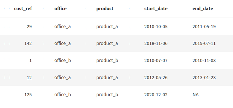
To perform the analysis, we need to transform the data to tell us the time for which each customer was active, and whether or not they have churned. To calculate the time for which the non-churning customer has currently been active, we have replaced the NA value with 2020-12-31, the date the data was (hypothetically) exported:
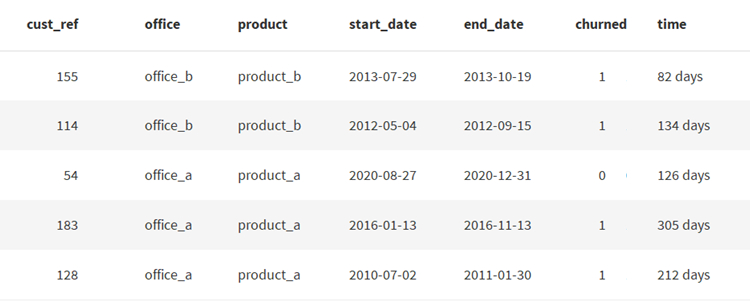
With the data in this format, we can perform our survival analysis. For this example, we’ll use a model called the Kaplan-Meier analysis, but other survival models, including the Cox and Weibull models, can also be used, with the appropriate model chosen on the basis of the dataset’s characteristics.
Choosing an appropriate model for the data is an important step of the process, but is outside the scope of this post. If you are interested in exploring this further, there are some excellent resources online (or you can contact us and we can talk data distributions and model assumptions!).
If we create a Kaplan-Meier model using our sample dataset and plot the results, we can see how the proportion of retained customers falls over time. The small vertical lines on the graph indicate our censored observations; in this case, those that are current customers at that particular time:
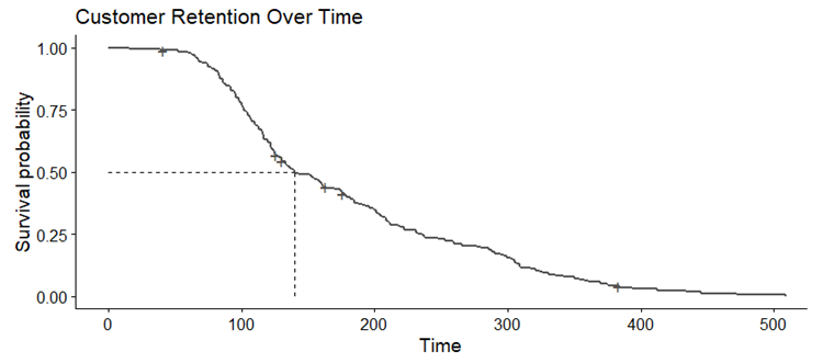
We can clearly see that customer churn is quite flat for around the first 75 days or so before a period of faster churn, with 50% of customers having churned by just under five months post-start. The rate of churn then slows, with a long “tail” of customers continuing to past 500 days.
Looking at this result, we might start to look at that point in the line where the churn begins to accelerate. Is there some way can intervene at this point to remind customers of the benefits, or offer an incentive to subscribe for a fixed time period?
From reporting to insight
Although the overall survival curve reveals much about how customers churn over time, we’re not yet taking advantage of all the features available in our dataset. By considering each sales office separately, we can observe if different offices are associated with longer or shorter customer retention times:
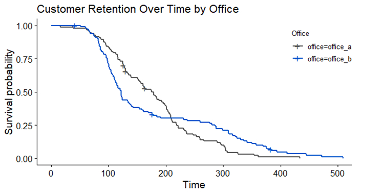
This survival analysis should provoke plenty of discussion. It appears that office_a shows faster churn early, but with a longer tail for longer retention times, whereas office_b exhibits a more steady rate of churn.
But note that the survival lines cross. This is a warning sign telling us that the assumptions for this model may not have been met (we’ll save a discussion of non-proportional hazards for another post!). In other words, we can’t simply answer the question “Which office is best at customer retention?” as the answer changes depending on what time of the customer engagement we are talking about.
The crossing lines do, however, encourage us to do some further digging into the data. If we look at the survival curves for the two products, we get this result:
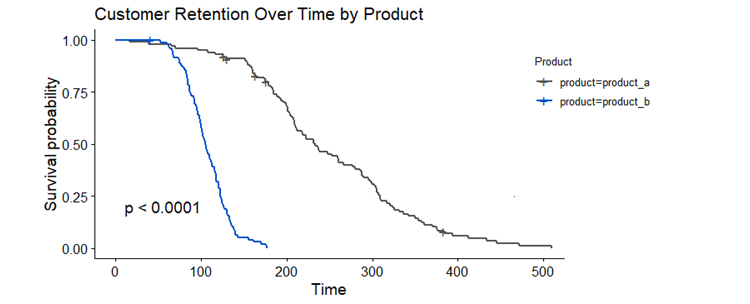
We can see a clear difference in customer retention time by product, with strong statistical confidence that our customer lifespan is different for our two products. Can this shed some light on the performance differences between offices?
If we look at how each office breaks down by the proportion of customers signed up to each product, we can see that office_b has a higher proportion of customers on product_b. This is the product we already know to be associated with faster customer churn.
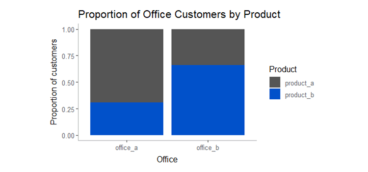
This result explains the shapes of the survival curves we saw when we compared office performance. The higher proportion of product_b customers in office_b could be responsible for the early high rate of churn, with the curve flattening once the majority of product_b customers have churned.
If we now perform our survival analysis breaking down by both office and product, we can get a better understanding of how churn varies between products and offices:
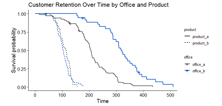
Although the two offices perform similarly in terms of customer retention for product_b, we now see that office_b seems to retain product_a customers for longer than office_a. That insight could then lead to additional hypothesis and investigations to identify the reasons for this, which could in turn lead to improvements in performance across the organization.
Survival analysis in marketing
Survival analysis is a great technique for performing time-to-event analysis. In many use cases, a survival analysis makes better use of the data than methods such as regression. It can also be used for descriptive reporting and to generate hypotheses to test using other methods.
Admittedly, the example we’ve put together is quite simplistic, and we haven’t discussed model selection, assumptions we need to make about the dataset, or statistical significance testing. If you’re interested in learning more about using R to perform survival analysis, you can’t go wrong with this excellent tutorial.
For marketers, breaking down a survival analysis across customer cohorts can provide valuable insight. For example, imagine we have a video subscription service and need to understand customer lifetime value (CLV) so we can determine a break-even cost per acquisition to inform our paid search activity. If we have been passing our acquisition channel data from our web analytics data to our CRM database (get in touch if you’re not, but you want to!), we can break down our survival curves by channel, campaign, or even matched keyword.
We may find that subscribers who joined from “action films” campaigns remained subscribers for longer than those who joined from “classic films” campaigns and we can adjust our bid strategies appropriately. We may also then discuss this finding with our video content team, who may look at whether more classic films need to be available, improving the experience of those subscribers (and hopefully their CLV).
Of course, survival analysis doesn’t only have to focus on loss. While we’ve focused on churn, remember that we can refer to a survival analysis as a time-to-event analysis. Why not turn it on its head and analyze time to conversion? You can identify which channels and which email sequences are associated with faster lead-to-customer transitions, allowing you to test and optimize your lead-nurturing strategies.
In short, there are myriad insights and opportunities that can be uncovered using survival analysis. To start applying such insights to your business, get in touch with Proove.
